

Livestock Units calculation: a method based on energy needs to refine the study of livestock farming systems
Head
The concept of a livestock unit (LU), which was originally intended to reflect the animal stocking rate on the farm according to the energy requirements of the animals, is now based on standardized coefficients that do not take into account certain essential characteristics of the animals, such as their size or production level. To take these characteristics into account, we propose equations for calculating livestock units based on the net energy requirements of animals and usable at the farm level.
Introduction
The concept of an animal unit appeared at the beginning of the 20th century in the United States to better appreciate the use of pastures used simultaneously by cattle and sheep (Scarnecchia, 1985). The animal unit then reflected the grass harvesting capacity of a grazing herbivore, with one adult cow considered to be worth one horse, five sheep or five goats. Additionally, in the United States, in the mid-1950s, the animal unit was explicitly defined on the basis of the animal's live weight but implicitly referred to the level of forage intake on pasture. In France, the livestock unit (LU) concept appeared in the early 1960s to help analyse production systems (Boichard, 1969), with the aim of enabling comparisons between herds of different structures based on the animals' energy requirements (Coléou, 1960). In the United Kingdom, Upton (1989) expresses the fact that the evaluation of the productivity of a herd must be expressed per animal, thus leading to the consideration of the different types of animals in this herd and to their expression in a common unit. Coefficients for conversion into LUs were then proposed basis of the energy requirements of the animals, which depend solely on the animal's metabolic weight. In the 1980s, to characterise and develop livestock farming in the African tropics, the first task was to quantify the number of animals present in these regions by aggregating large and small ruminants and monogastric animals. The concept of the tropical livestock unit (TLU) was thus proposed (Jahnke, 1982). It was then important to evaluate the number of ruminants in relation to the available rangeland and pasture areas, hence the concept of the tropical cattle unit (TCU).
Regardless of the method of extrapolation between types of animals or species, the notion of animal unit requires the definition of a reference animal. In Australia, this is the empty sheep (McLaren, 1997). In the United States, in 1974, the Society for Range Management defined an animal unit corresponding to a dry pregnant cow weighing 1000 pounds (454 kg live weight) and consuming 12 kg of dry matter (DM) of forage per day, without specifying any further details on the high qualitative variability between types of forage. There was some discussion about the relative importance of animal weight and forage intake in defining an animal unit. Scarnecchia and Kothmann (1982) proposed to base the definition on forage intake only (1 animal unit = 12 kg DM forage/day). In Africa, for Upton (1993), an LU is a cow (female over 4 years old) of 250 kg, and the equivalence coefficients of the different types of cattle are calculated according to the metabolic weight of the animals (1 heifer from 1 to 4 years old weighing 100 kg =0.50 LU; 1 whole or castrated adult male of 320 kg =1.20 LU). In the tropics, a TLU is defined on the basis of an animal weighing 250 kg regardless of its type, age or sex; this definition coexists with that of a TCU represented by a bovine weighing 175 kg (1 TCU =0.70 TLU). A flat live weight, and therefore a TLU coefficient, is assigned to small ruminants (25 kg or 0.10 TLU), mules (175 kg or 0.70 TLU), pigs (50 kg or 0.20 TLU) or poultry (2.5 kg or 0.01 TLU) (Jahnke, 1982; Assouma et al., 2018).
In France, LU was defined as a unit of net energy consumption by zootechnicians, and its initial definition (in the 1960s) was clear: an LU corresponded to a 600 kg dairy cow producing 3 000 kg of milk and consuming 3 000 feed units (UF Leroy, 1 UF = energy content of one kilo of barley (Demarquilly et al., 1996)) per year. Over the years, depending on the needs of the various technical, economic or administrative services for the analysis of livestock production systems, the definition of the LU has shifted from an energy consumption level, which is difficult to assess, to a standard fodder consumption level, defined on the basis of 4 500 kg DM of fodder per year. This "sliding" French definition of the LU was finally fixed and collectively adopted empirically by the agricultural profession and the Centre d'Economie Rurale (Iger-Centres-de-Gestion, 1989): it is a dairy cow with a live weight of 600 kg, a production level of 3 000 kg of milk per year, an annual requirement level of 3 000 FU and an annual forage consumption of 4 500 kg DM.
In reality, these levels of forage consumption (and a fortiori of UF) are not available because they are very difficult to evaluate, especially for the grazing period. Moreover, it no longer seems appropriate to estimate the LU value of a herd on the basis of the level of forage consumption when concentrate consumption can reach two tons per cow per lactation in well-referenced production systems (Idele, 2019). Additionally, in the absence of available data on animal intake levels, technical-economic analyses are generally based on the equivalence of 1 cow =1 LU, particularly for calculating the stocking rate of the fodder area, for extremely variable levels of requirements and forage use by animals. Three limitations appear when the LU coefficient is based on a standard quantity of forage dry matter consumed: i) the high variability of forage digestibility and of their share in the ration; ii) concentrate inputs can represent a very large share of the energy and protein requirements of animals with high needs; iii) since forages are primarily intended for herbivores, a notion of LU based on their consumption does not allow for the extension of an Animal Unit system to monogastric animals.
In addition to its use in research and development for the analysis of production systems, the LU concept is widely used for statistical purposes and for administrative management, such as the payment of public aid. A certain convergence of LU values for a given type of animal exists between the different actors or institutions, but differences can be important, particularly for small ruminants (Table 1).
Table 1. LU coefficients used for different types of animals in cattle, sheep and goat herds in France according to various institutes and users and in European statistics (for a one-year presence of the animals) (EUROSTAT, 2019, IDEA, 2019).
Research |
Institut |
Administration |
Eurostat |
|
|---|---|---|---|---|
Dairy cow |
1.0 |
1.0 |
1.0 |
1.0 |
Suckler cow without calf |
0.86 |
0.85 |
1.00 |
0.80 |
Female 3-8 months |
0.32 |
0.25 |
0.00 |
0.40 |
Female 8-12 months |
0.39 |
0.40 |
0.60 |
0.40 |
Female 12-24 months |
0.60 |
0.60 |
0.60 |
0.70 |
Female 24-36 months |
0.80 |
0.80 |
1.00 |
0.80 |
Male 3-8 months |
0.32 |
0.25 |
0.00 |
0.40 |
Store male 8-12 months |
0.45 |
0.40 |
0.60 |
0.40 |
Store male 12-24 months |
0.65 |
0.60 |
0.60 |
0.70 |
Young bull 8-12 months |
0.45 |
0.60 |
0.60 |
0.40 |
Young bull 12-24 months |
0.80 |
0.80 |
0.60 |
0.70 |
Steer 8-12 months |
0.45 |
0.45 |
0.60 |
0.40 |
Steer 12-24 months |
0.65 |
0.60 |
0.60 |
0.70 |
Steer 24-36 months |
0.85 |
0.80 |
1.00 |
1.00 |
Ewes |
0.14 |
0.15 |
0.15 |
0.1 |
Lamb less than 6 months old |
0.05 |
0.05 |
0 |
|
Ewe lamb over 6 months old |
0.07 |
0.07 |
0.15 (>1 year) |
|
Ram over 6 months |
0.10 |
0.15 |
0.15 |
|
Lamb for slaughter |
0.05 (0.06-0.09) |
0.05 |
0 |
|
Goat |
0.18 |
0.17 |
0.15 |
0.1 |
Femal kid (3 months to a year) |
0.08 |
0.09 |
0.15 |
|
Billy goat |
0.18 |
0.17 |
- |
An important limitation to the use of the LU in the different countries that use this concept for technical-economic analyses is the fact that, for a given animal category, the LU coefficient per animal is constant regardless of its size or production level, which can bias the conclusions of zootechnical or economic studies using the LU in the construction of indicators for analyses. Some authors have thus been led to make corrections for variations in animal feed requirements in the analysis of livestock systems over different time horizons (Cavailhès et al., 1987). It should be remembered that these indicators are most often aimed at quantifying the animal "load" on the farm, on the scale of an agricultural year (12 months), with regard to the production factors used (whether it be land and fodder resources, labour, capital, etc.) on the one hand, and the production marketed on the other.
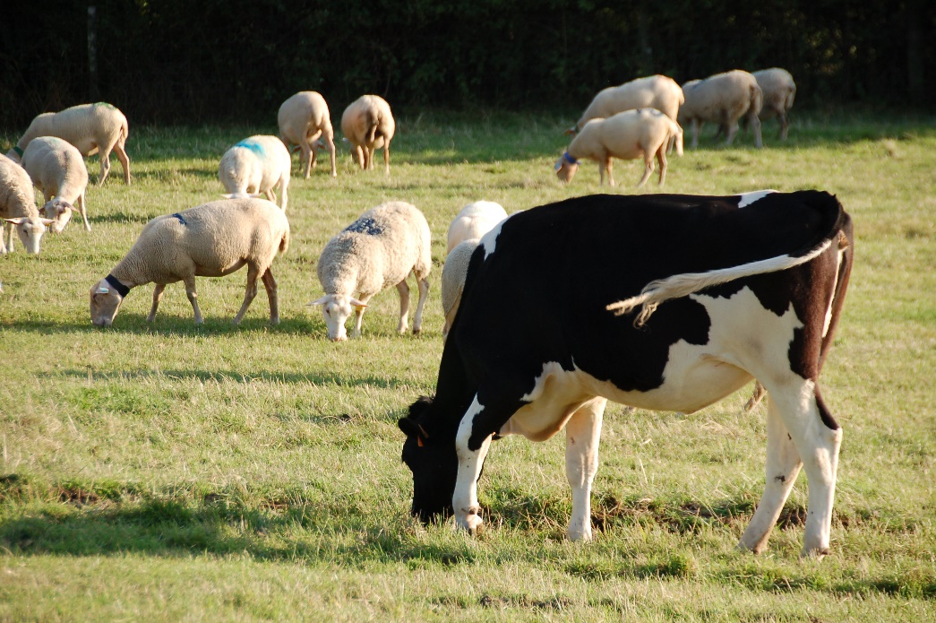
The objective of this paper is to propose a method for calculating the LU according to the descriptive data of the animals (Rothman-Ostrow et al., 2020), taking simultaneously into account their size and their production level. For this, a metric is needed, and we retain the net energy requirements of the animals. This proposal seems to us essential for accurate, comparative (between farms, especially for farms raising different animal species, photo 1) or diachronic technical-economic analyses; indeed, the "weight" of the herd appears to be central for correctly evaluating both the efficiency of the means of production used and the levels of production. The LU remains an indispensable concept in works developed at 'meso' perimeters: not at the scale of an animal or a batch of animals, nor at the scale of a large region or a country, but at the scale of a farm or a group of farms.
Photo 1: Cattle and sheep from the INRAE Herbipôle herd in mixed grazing on the Puy de Berzet (Photo credit: Marc Benoit).
After presenting our proposals and our methodological choices, which are intended to be generic, i.e., applied in various and contrasting production contexts, we make a proposal for calculating LUs for cattle, sheep and goats on a herd scale. A sensitivity analysis for each parameter selected and taken independently in this calculation method leads us to propose two types of equations according to the information available and whose level of precision will be different. Finally, we will discuss the selected method as well as the results of the application of the two methods to contrasting case studies in dairy cattle and sheep for meat productions.
1. Methodological proposal
1.1. A method based on the net energy requirements of animals
After the first proposals to base the concept of livestock units on the energy requirements of animals, the level of fodder intake became, for ease of implementation, the central element of the definition of the livestock unit. However, since the 1950s, with higher production targets and in parallel with the progress made in animal selection and feeding, the energy requirements of animals became the main criterion for characterizing an animal, with the increased use of concentrates to supplement fodder and the development of techniques to improve their value (grass and maize silage in particular). Moving from dry matter intake to gross energy ingested by animals requires knowledge on the composition of rations throughout the year. Moreover, moving from gross energy to net energy requires precise knowledge of feeds, particularly in terms of digestibility (Demarquilly et al., 1996; INRA, 2018). These elements are impossible to apprehend at the scale of the different periods of the year and the various types of animals composing the herd. This leads us to propose to base the calculation of the LU on the total annual net energy requirements (NEt) of the animals, calculated from the equations used by the IPCC (Intergovernmental Panel on Climate Change, 2019) at the Tier 2 level, i.e., at a high level of accuracy. This level represents a good compromise with respect to our objectives: to account for the physiological stage (gestation, lactation, growth, etc.), the rearing method (free-range, building), the size and the production level of the animals while being based on parameters accessible in on-farm surveys. This means considering both the energy requirements for the maintenance and activity of the animals and the requirements for production and growth and even work. We can also keep the notion of a standard animal (dairy cow close to that defined in the historical method, with a production of 3 000 litres of milk per lactation) by calculating its total net energy requirements (NEt). This animal will represent one LU and will allow us to transform the net energy requirements resulting from the equations proposed for each type of animal considered into LU equivalents.
1.2 Calculation of net energy requirements of ruminants
The IPCC, as part of the study of climate change, describes a method for calculating GHG (greenhouse gas emissions) from livestock and their effluents (IPCC, 2019). This calculation leads to defining the energy needs of livestock in terms of net and gross energy to estimate their intake of fodder. The Tier 2 approach requires specifying, for a type of animal, the zootechnical factors of variation in its energy requirements, in particular its production level and its weight, through the concept of metabolic weight (kg of live weight at power 0.75). Used since the 1930s, this concept is transversal and applicable to the entire animal kingdom (Blaxter, 1989). Basal metabolic energy ("maintenance needs") is proportional to metabolic weight, although it also depends on environmental conditions, physiological state, etc. (Ortigues, 1991). The other major element of the proposed method is the consideration of the animal's production level (milk production or weight gain).
The IPCC proposes equations for calculating energy requirements for the various types of animal needs, as shown in Table 2 and detailed in Appendix 1. We do not include the energy requirements for cattle work (Equation 10.11), including traction, or the energy required to regulate the temperature of the animals during the cold season (Equation 10.2), due to the availability of data and/or the fact that this is not common practice in Europe. The main variables used in these equations are presented in Table 2.
Table 2. Different types of net energy requirements of animals, equations proposed by the IPCC and variables needed to calculate them.
Net energy requirements for: |
IPCC equation no. |
Required variables |
|---|---|---|
Maintenance |
10.3 |
Live weight |
Activity |
10.4-10.5 |
Live weight, type of pasture: plain, mountain, rangeland |
Growth |
10.6-10.7 |
Live weight, adult weight and daily weight gain |
Lactation |
10.8-10.9-10.10 |
Quantity of milk produced, fat and protein content |
Work |
10.11 |
Not taken into account |
Wool production |
10.12 |
Quantity of wool produced, for small ruminants |
Gestation |
10.13 |
Live weight and prolificacy for small ruminants |
IPCC equation numbers correspond to the numbers published in the IPCC (2019).
1.3 Calculation of the herd's LU value
The energy requirements calculated according to the IPCC equations are expressed in MJ per day. The concept of LU is linked to an annual presence of each category of animals and therefore to an annual consumption of NEt. For animals present on the farm throughout the year (cows, ewes, goats), we calculate the sum of daily needs by subperiods composing the annual campaign, according to the physiological stage of the animal (dry, in production, pregnant), its production (milk or meat), its activity, linked to the type of grazing and the housing mode. For the animal categories present for a fraction of the year, we calculate the NEt requirements over the period by summing the daily requirements. These requirements are then expressed for a period of one year by dividing them by the number of days of the presence period and multiplying by 365. These annual NEt requirements are then divided by the NEt requirements of the reference animal counting as an LU to obtain the LU value for the type of animal considered. The NEt requirement is not calculated individually (per animal) but for each category of animal in the herd using the average zootechnical characteristics of the batch. The size of the herd in LUs is calculated by summing the LU values of the different categories of animals, which are themselves the product of the average annual number of animals (based on the monthly or, better, daily number of animals) and the LU coefficient for the same category.
1.4. Reference animal counting as one livestock unit
We propose to base the characteristics of the reference animal on the average dairy cow used as a historical reference in France, i.e., a 600 kg cow producing 3 000 kg of milk at 4% fat in one year. We consider that this average cow spends half the year in pasture and the other half in stalls, that she produces one calf per year with a lactation period of 305 days and a dry period of 60 days and that she benefits from constant thermal comfort throughout the year. This cow is in a herd with a renewal rate of 22%, whose primiparous cows calve at 3 years of age, at 95% of adult live weight. According to the IPCC equations, such an average cow has an annual NEt requirement of 29 000 megajoules (MJ). We use this basis to define one LU.
1.5. Approach to the construction of equations for estimating the NEt requirement
For very fine approaches, it is possible to systematically use the IPCC equations if all the necessary parameters are available, which is rarely the case. We first considered all the animal characterization variables necessary to calculate its energy requirements (Table 2) and a priori accessible on the farm for the bovine, ovine and caprine species. We thus calculated the NEt and the LU coefficient of an "average" animal in the context of current European livestock production by qualifying this animal as "pivotal" for each of the three species and by distinguishing between milk and meat production for cattle. In a second step, a sensitivity analysis was carried out in each of these cases to identify the variables that have the greatest influence on the NEt result. For this purpose, minimum and maximum values are proposed for each variable, based on the references made available by the Institut de l'Elevage on all ruminant breeding systems in France, taking into account more particularly the most extreme production systems in terms of animal size, production levels and rearing method. For each variable, we calculate the ratio between the range of variation of the LU value induced by its own variation (between its minimum and maximum values) and the pivotal value retained, the level of the latter thus having only an indicative value and not influencing the result of the sensitivity analysis. We vary each of the variables one by one, with the value of the other variables remaining fixed. This process allows us to identify the variables that most influence the NEt result, all other things being equal. By expertise, we can then determine the variables that we fix (standardization) as having a lower impact on NEt, with a view to proposing two types of equations ("basic proposal" or "simplified") depending on the context and the availability of data.
2. Application to bovine, ovine and caprine species
Table 3 lists the equations we propose for calculating net energy requirements, depending on the type of animal considered and the length of time it is kept.
Table 3. Summary of equations and tables proposed for calculating net energy requirements of animals, by species, type of animal, period considered, according to two levels of precision.
Species |
Equation |
Type of animal |
Period |
Type of equation |
|---|---|---|---|---|
Dairy cattle |
(1) |
Cow |
1 year |
Basic proposal |
(2) |
Cow |
1 year |
Simplified |
|
Suckler cattle |
(3) |
Cow + calf less than 3 months old |
1 year |
Basic proposal |
(4) |
Cow + calf less than 3 months old |
1 year |
Simplified |
|
Cattle |
(5) + Tables 5 and 6 |
Heifers |
1 year |
Basic proposal |
(6) |
Males, all ages |
1 year |
Basic proposal |
|
Sheep |
(8) |
Ewes + lambs before weaning |
1 year |
Basic proposal |
(9) |
Lambs after weaning |
1 year |
Basic proposal |
|
(10) |
Ram |
1 year |
Basic proposal |
|
(11) |
Ewes + lambs before weaning |
1 year |
Simplified |
|
(12) |
Lambs after weaning |
1 year |
Simplified |
|
(13) |
Ewes + lambs + rams |
1 year |
Simplified |
|
(14) |
Lambs for fattening |
Fatt. period |
Basic proposal |
|
Table 9 |
Lambs for fattening |
Fatt. Period |
Simplified |
|
Goats |
(15) |
Goats and kids |
1 year |
Basic proposal |
(16) |
Goats and kids |
1 year |
Simplified |
|
(17) |
Goat |
1 year |
Basic proposal |
|
(18) |
Goats, kids and billy goats |
1 year |
Simplified |
|
(19) |
Fattening kids |
Fatt. Period |
Basic proposal |
|
Table 10 |
Fattening kids |
Fatt. Period |
Simplified |
2.1. Cattle
a. Dairy cows:
An "average" French dairy cow was selected (Idele, 2020a), weighing 640 kg, producing 7 000 kg of milk per 340-day lactation at 4% fat, grazing 4 months per year, with a calving-calving interval of 420 days and a dry period of 65 days (Idele, 2020a). This cow is in a herd with a 33% turnover rate, and the primiparous cows calve at 30 months (at 93% of adult live weight). Such a cow has a NEt requirement of 41 800 MJ per year (51% for lactation, 42% for maintenance, 4% for pregnancy, 2% for activity and 1% for growth), which corresponds to 1.44 LU (41 800/29 000). This value is called the "pivot value". A production of 7 000 kg of milk per cow per year corresponds to the average production of European dairy cows (from 5 900 kg/cow/year in Ireland to 9 900 kg/cow/year in Denmark), and the world average milk yield of cows is 2 500 kg per year (from 1500 kg/cow/year in India to 10 600 kg/cow/year in the USA). The range of variation of the values of each variable taken into account to calculate NEt is determined according to observable realities in France (Idele, 2020c). Figure 1a shows the impact of the minimum and maximum values of each variable considered on the LU value around the "pivot" value. It appears that the quantity of milk produced and the weight of the cows are the two variables with the greatest influence on the LU value. Then, comes the fat content of milk and the length of the grazing period. The other variables (calving-calving interval, lactation length, weight of primiparous cows at calving and turnover rate) have little impact on the NEt requirements.
Figure 1: Variations in the LU coefficients of dairy cows (a) and suckler cows (b) generated by the variation of the variables used to calculate net energy requirements between the minimum and maximum values adopted.
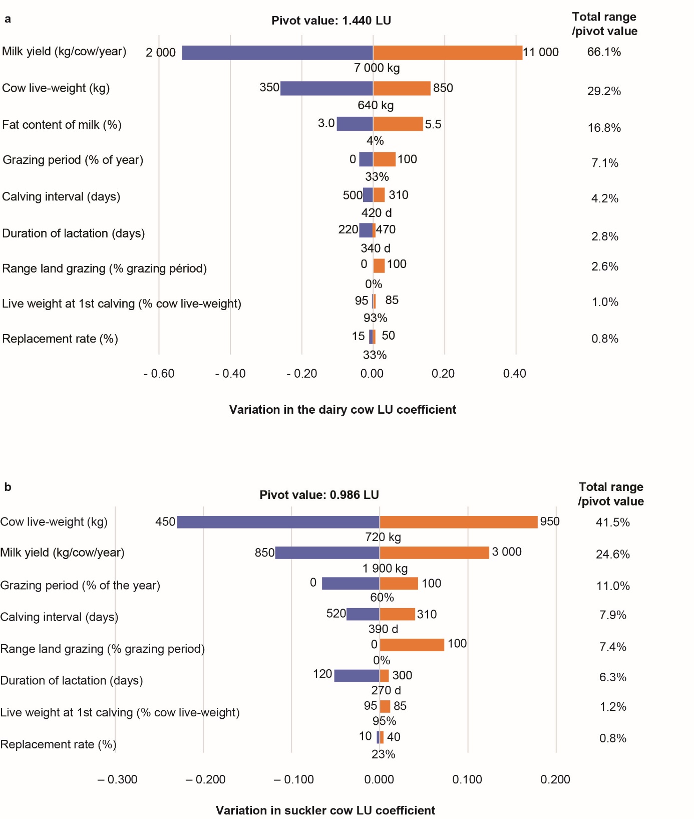
Variables ranked in descending order of impact on the pivotal LU value defined for an average animal whose characteristics are specified as the central value of each variable (e.g., milk production of 7 000 litres per dairy cow).
We propose to retain the four variables that have the most weight in the sensitivity analysis (milk production, live weight, milk fat content and length of grazing period) to which we add the time spent grazing on pasture, which is combined with the length of the grazing period. To reduce the calculation to a one-year presence time, we set the lactating cow's presence time at 81% (340 days of lactation for a 420-day calving interval) and therefore 19% of her presence time as dry and 0.87 pregnancies per cow per year (420-day calving interval). This allows us to propose the following equation for the annual NEt requirement of a dairy cow:
(1) ENt_DC (MJ/yr)=(DP×(22.7+25.4×GR)+148.3)×LW0.75+(1.47+0.40×FC)×QM
where DP = duration of the grazing period expressed as a share of annual time (from 0 to 1), GR = share of grazing time spent on rangelands or large mountain areas (from 0 to 1), LW=live weight of the cow in kg, FC=milk fat content in %, and QM = quantity of milk produced per cow in kg per year.
The variables LW and QM are relatively easy to collect by survey or consultation of technical databases. If the FC variable is not available, we propose to set it at 4%; if the length of the grazing period is unknown, we propose to set the time spent grazing and in stalls at 33% and 67% of the year, respectively. Thus, the simplified Equation (2) considers only the two variables that have the most weight (LW and QM) and are also the most accessible.
(2) ENt_DC (MJ/yr)=156×LW0.75+3.07×QM
b. Suckler cows
The average animal is a French suckler cow (France has one-third of the European suckler cow herd) of 720 kg that produces 1 900 litres of milk (Sepchat et al., 2017) sucked by her calf for 270 days. Her calving interval is 390 days (Idele, 2020d), and her dry period is 120 days. Few references exist on the fat content of milk from suckler cows, which we set at 45 g per kg of milk (Sepchat et al., 2017). As suckler farming is mainly grazing, this cow grazes 7 months a year. She is in a herd with a replacement rate of 23%, with primiparous cows calving at 36 months (at 95% of adult live weight). She thus has an NEt requirement of 28 600 MJ per year (65% for maintenance, 21% for lactation, 7% for activity, 6% for pregnancy and 1% for growth), which corresponds to 0.99 LU (28 600/29 000). The live weight of the cows and their milk production are the most important factors (Figure 1b) in the calculation of NEt. The energy requirements for the activity of suckler cows are relatively more important (7% of NEt) than those of dairy cows and are influenced by the length of the grazing period and the type of grazing (paddock, rangeland, and mountain areas). We thus propose to keep the three variables that have the most weight in the sensitivity analysis (Figure 1b): live weight, milk production and duration of the grazing period for the calculation of the NEt requirements of a suckler cow (Equation (3)), to which we add the variable grazing time on pasture that is combined with the variable duration of the grazing period. To reduce the calculation to a one-year attendance time, we set the lactating cow's attendance time to 69% (270 days of lactation for a calving interval of 390 days) and the number of pregnancies per cow per year to 0.94 (390 days of calving interval).
(3) ENt_SC (MJ/yr)=(DP×(22.7+25.4×PP)+146.2)×LW0.75+3.27×QM
where DP = duration of the grazing period expressed as a share of annual time (from 0 to 1), PP = share of grazing time spent on rangelands or large mountain areas (from 0 to 1), LW=live weight of the cow in kg, and QM = milk production of the cow in kg/year.
Milk production is difficult to estimate for suckling cows. It can be approximated by estimating that a calf drinks an average of 6 to 8 litres of milk per day over its lactation period (Sepchat et al., 2017). By knowing the average duration of calf suckling at the udder (which generally corresponds to the age at weaning of the calf, except in some cases where calves are separated from the mothers and fed reconstituted milk while the cows are dry), we can estimate the total milk production of the cow (QM=milk drunk by calves in litres per day x duration of suckling at the udder in days). We also estimate the duration of the grazing period by setting it at 60% of the annual attendance time. Thus, we propose the simplified Equation (4):
(4) ENt_SC (MJ/year) =160×LW0.75+25×Suck
where LW = live weight of the cow in kg, Suck = duration of dam suckling calf in days
c. Heifers for breeding and fattening
Breeding heifers are growing animals intended for herd renewal and calving at two to three years old. Their NEt requirements are the sum of their maintenance, activity, growth and pregnancy requirements. They depend on the animal's live weight and daily weight gain, which leads to the definition of key life periods for which NEt requirements are calculated. Each period is characterised by the beginning and end live weights and therefore an average weight gain for the animal considered, objective set by the breeder to reach a sufficient weight at the time of calving. The growth requirements depend on the age at calving, the objective being in general to reach 85 to 95% of the weight of the adult cow. From their second week of life, female calves in the dairy herd receive fodder and concentrates in addition to milk, which is often reconstituted from powder with a high proportion of plant proteins; from birth to three months of age, we consider that the NEt requirements of dairy heifers are covered on average by 50% by nondairy feed. These dairy heifers are weaned between 2 and 3 months of age; from 3 months of age, their energy requirements are met 100% by solid feed (forages and concentrates). Heifers in suckler systems are weaned between 4 and 9 months. In general, they do not consume any fodder or concentrate from 0 to 3 months of age and therefore count as 0 LU during this period. At three months, 20 to 30% of the needs of these heifers are covered by feed other than mother's milk (Idele, 2014b). We therefore consider that over the period from 3 to 8 months, their NEt needs are covered at 60% on average by forages and concentrates. Table 4 sets weight targets as a percentage of adult cow weight for different typical heifer ages.
Table 4. Liveweight targets dairy and suckler heifers as a percentage of mature cow weight at different typical ages by age at calving.
Heifers |
Typical ages |
3 months |
6 months |
12 |
24 |
30 |
36 |
|---|---|---|---|---|---|---|---|
Calving 2 years |
15 |
30 |
50 |
85 |
- |
- |
|
Calving 30 months |
43 |
78 |
93 |
- |
|||
Calving 3 years |
43 |
70 |
- |
95 |
|||
Heifers |
Typical ages |
3 months |
8 months |
12 months |
24 months |
30 months |
36 months |
Calving 2 years |
20 |
45 |
58 |
85 |
- |
- |
|
Calving 30 months |
20 |
43 |
51 |
81 |
93 |
- |
|
Calving 3 years |
20 |
40 |
51 |
75 |
- |
95 |
In all equations for calculating energy requirements, the live weight of heifers can be expressed in terms of the live weight of the mature cow. For example, the average live weight of a 1-2-year-old dairy heifer calving at 3 years of age will be, according to Table 4: (0.43×LWC+0.70×LWC)/2, where LWC is the live weight of the adult cow. The weight gain between 1 and 2 years of age of this same heifer will be 0.70×LWC-0.43×LWC. The only weight variable used in IPCC Equations 10.3 and 10.6 is the live weight of the adult cow. We assume that all heifers spend half the year on pasture and half the year in the barn, except for dairy heifers, which remain in the barn for up to six months. Pregnancy requirements are calculated over the last 9 months before calving. Combining Equations 10.3, 10.4, 10.6 and 10.13 of the IPCC, we obtain Equation (5) of the NEt requirement of a farmed heifer expressed only as a function of the weight of the adult cow:
(5) NEt_H (MJ/year)=a×LWc0.75+b×LWc1.097
where a and b are coefficients depending on the calving age of the heifer and the lifespan (Table 5), and LWc is the live weight of the mature cow in kg.
Table 5. Values of coefficients a and b for calculating the total net energy requirement of a breeding heifer as a function of its age at calving and length of life.
Heifers |
Periods of life |
0-3 months |
3-6 months |
6-12 months |
12-24 months |
24-30 months |
24-36 months |
|
|---|---|---|---|---|---|---|---|---|
Calving 2 years |
a |
64.14 |
103.72 |
- |
- |
|||
b |
2.71 |
3.46 |
- |
- |
||||
Calving 30 months |
a |
11.76 |
41.66 |
59.88 |
95.54 |
123.83 |
- |
|
b |
0.44 |
2.75 |
1.57 |
3.19 |
3.50 |
- |
||
Calving 3 years |
a |
59.88 |
83.10 |
- |
120.56 |
|||
b |
1.57 |
2.28 |
- |
2.78 |
||||
Heifers |
Periods of life |
0-3 months |
3-8 months |
8-12 months |
12-24 months |
24-30 months |
24-36 months |
|
Calving 2 years |
a |
32.93 |
77.52 |
108.29 |
- |
- |
||
b |
2.17 |
3.17 |
2.72 |
- |
- |
|||
Calving 30 months |
a |
0 |
32.17 |
72.39 |
101.98 |
125.46 |
- |
|
b |
0 |
1.93 |
1.74 |
2.87 |
2.77 |
- |
||
Calving 3 years |
a |
31.01 |
70.65 |
90.17 |
- |
123.29 |
||
b |
1.60 |
2.40 |
2.17 |
- |
2.22 |
|||
Suckler heifers intended for slaughter are fed with breeding heifers, except during their last three to four months when they receive a fattening ration. During this last period, the NEt requirement can also be expressed as a function of the adult cow's weight (target live weight of the heifer at slaughter: 90 to 105% of the live weight of the adult cow) with the coefficients a and b given in Table 6.
Table 6. Values of coefficients a and b for calculating the total net energy requirement of a beef heifer during its fattening period.
Heifer < 24 months |
30 months old heifer |
Heifer > 30 months |
|
|---|---|---|---|
a |
104.31 |
117.34 |
117.83 |
b |
4.04 |
4.13 |
3.62 |
For rearing periods, refer to the coefficients for rearing heifers calving at 24 months, 30 months and 36 months for beef heifers under 24 months, 30 months and 36 months, respectively.
d. Males
There is great diversity in the type of males produced, depending on whether they are castrated (steers) or not (weanlings, bulls, young bulls), their age at sale (from two weeks for dairy calves to more than 3 years for some steers), their weight at sale and therefore their daily weight gain (from less than 300 g to more than 1 800 g per day). For high-growth categories of animals (heavy weanlings, baby beef), production routes are relatively standardized: growth targets and sale ages differ little between countries, systems and cow breeds (Office de l'Élevage, 2008; Idele, 2010; Pesonen et al., 2013; Murphy et al., 2018). Whether derived from purebred cows (Charolaise, Limousine, Angus, Blanc Bleu Belge, Hereford, etc.) or from crosses with dairy breeds, these bull calves are sold between 15 and 20 months of age with 1 100 to 1 500 g average daily gains from weaning to sale.
For the categories of animals with lower growth rates (steers, store males), the types of animals are relatively diversified: in the grassland plains of South America, these males have low growth rates (300 to 500 g per day) and are slaughtered relatively light, between 350 and 500 kg (Pravia et al. 2014; Lampert et al. 2020); in European grassland areas, the steers produced have sufficient grass in quantity and quality to allow better growth and they are slaughtered heavier, from 650 to more than 850 kg (Réseaux d'élevage, 2005; Drennan and McGee, 2009; Taylor et al. 2018).
As with heifers, the live weight of males can be expressed as the live weight of the adult male (Table 7) in all energy requirement equations. The weight of the adult male is not available on the farms, as males are generally sold before they reach adulthood. We can estimate this weight relative to that of cows, considering that an adult bovine male weighs 40 and 50% more than a cow for suckler and dairy breeds, respectively. We obtain Equation (6) of the NEt requirement of a male, expressed only as a function of the weight of the adult male:
(6) NEt_Male (MJ/year)=a×LWm0.75+b×LWm1.097
where a and b are coefficients depending on the type of male produced and the period of life (Table 8), and LWm is the live weight of the adult male in kg.
Table 7. Liveweight targets for dairy and suckler males as a percentage of adult male weight at different typical ages according to the type of male produced.
Males |
Typical ages |
3 |
8 |
12 |
20 |
24 |
30 |
36 |
44 |
|---|---|---|---|---|---|---|---|---|---|
Store (weanling, |
14 |
30 |
41 |
- |
60 |
72 |
83 |
100 |
|
Fattened bulls |
14 |
33 |
48 |
80 |
- |
- |
- |
- |
|
Steers < 30 months |
13 |
30 |
40 |
- |
62 |
73 |
83 |
95 |
|
Steers > 30 months |
65 |
80 |
- |
- |
|||||
Males (dairy |
Typical ages |
3 months |
6 months |
12 months |
24 months |
30 months |
36 months |
||
Veal for slaughter |
14 |
25 |
33 |
- |
- |
- |
- |
- |
|
Store |
15 |
25 |
40 |
60 |
72 |
83 |
100 |
||
Fattened bulls |
16 |
27 |
50 |
82 |
- |
- |
- |
- |
|
Steers |
13 |
23 |
36 |
- |
54 |
- |
76 |
90 |
Table 8. Values of coefficients a and b for calculating the total net energy requirement of a male, depending on its type and length of life.
Males |
Periods of life |
0-3 |
3-8 |
8-12 |
12-24 |
24-30 |
24-36 |
36-44 |
|
|---|---|---|---|---|---|---|---|---|---|
Store |
a |
28.24 |
67.39 |
87.78 |
- |
113.93 |
137.09 |
||
b |
0.73 |
1.47 |
1.05 |
- |
1.68 |
2.27 |
|||
Fattened bulls |
a |
0 |
29.67 |
68.56 |
96.63 |
- |
- |
- |
|
b |
0 |
0.93 |
2.28 |
3.47 |
- |
- |
- |
||
Steers > 30 months |
a |
24.16 |
58.03 |
76.96 |
94.96 |
105.84 |
116.85 |
||
b |
0.88 |
1.50 |
1.42 |
1.75 |
1.77 |
1.74 |
|||
Steers < 30 months |
a |
24.16 |
58.03 |
78.65 |
100.19 |
- |
- |
||
b |
0.88 |
1.50 |
1.67 |
2.60 |
- |
- |
|||
Males (dairy |
Periods of life |
0-3 months |
3-6 months |
6-12 months |
12-24 months |
24-36 months |
36-44 months |
||
Veal for slaughter |
a |
11.55 |
19.81 |
26.68 |
- |
- |
- |
||
b |
0.30 |
0.65 |
0.95 |
- |
- |
- |
|||
Store |
a |
12.01 |
40.39 |
63.07 |
87.13 |
113.93 |
137.09 |
||
b |
0.35 |
1.19 |
1.24 |
1.10 |
1.68 |
2.27 |
|||
Fattened bulls |
a |
12.46 |
42.64 |
66.01 |
98.89 |
- |
- |
||
b |
0.41 |
1.39 |
2.25 |
3.55 |
- |
- |
|||
Steers |
a |
9.45 |
32.48 |
51.04 |
70.06 |
92.31 |
110.89 |
||
b |
0.61 |
1.26 |
1.13 |
1.04 |
1.71 |
1.95 |
|||
2.2 Sheep
Our objective is to calculate the LU value of the different types of animals making up the sheep flock (ewes, lambs, rams) but also of a “followed we”, i.e., with its lambs, its renewal and the share of associated ram. Indeed, the data most easily accessible in farm surveys are the overall number of breeding ewes, the replacement rate and ewe productivity (number of live lambs per ewe per year).
Ewe productivity is a determinant variable of the overall technical and economic performance of farms and is most often monitored in surveys (Benoit et al., 2019); therefore, it is usually available or estimable. Ewe productivity is calculated as follows (Benoit et al., 2020):
(7) Ewe Productivity (EP)=LR×Prol×(1-LbsMortality)
where LR is the average annual lambing rate of the flock (number of lambs per ewe per year), Prol is the average annual prolificacy of the flock (number of lambs born per lambing) and LbsMortality is the percentage of dead lambs among lambs born. Including the EP variable in our equations will therefore mean that the LbsMortality variable is also taken into account.
Litter weight at birth is a factor in ewe lactation requirements. This weight is dependent on the weight of the ewe and the prolificacy. According to Thériez (1991), we integrate in our model a relationship between the weight of the ewe and the weight of a single born lamb (Equation (a)), a relationship between the weight of a double born lamb and a single born lamb (Equation (b)), and finally, a relationship between the weight of a double born lamb and a triple born lamb (Equation (c)):
(a) LW1=0.00559×LWb+1.0377
(b) LW2=LW1×(1.7642–4.367×LW1×LWb0.75)
(c) LW3=0.846×LW2
where LWb is the weight of the ewe and LW1, LW2, and LW3 are the birth weights of single, double and triple lambs, respectively.
Equations (d), (e) and (f), established on a large database of lambing data (with prolificacies varying from 110 to 230%), give the proportions of single, double and triple lambs born according to the prolificacy level of the dam. Considering that the mortality of double and triple lambs is increased by 50 and 150%, respectively, compared to that of single lambs, we can finally estimate the average weight of lambs born. The latter allows us to calculate the ewe's milk production for the growth of her lambs, from birth to weaning (via the variable "Prol", Equation (8)), according to the equivalence of five litres of milk for one kg of weight gain (IPPC, 2019).
(d) % single_born_lambs=0.003×Prol2–1.7147×Prol+241.2
(e) % double_born_lambs=–0.0057×Prol2+2.2979×Prol–172.8
(f) % lambs_born_triple=100-(d)-(e)
To calculate the LU value of the flock, we propose, for sheep and goats, to consider all females from one year of age as constituting the flock of reproductive females. Indeed, theoretically, it would be necessary to distinguish ewe lambs (or goat kids, for goats) between one year and the age of their lambing, with specific LU coefficients. However, there is generally no individual monitoring of animals that would allow this, but above all, the net energy requirements of a pregnant ewe lamb added to its growth needs are globally little different from those of an ewe (with gestation, lactation and drying off phases). The "ewe lamb" category is therefore considered for the calculation of its LU value from weaning to one year of age. This value is then integrated with the “followed ewe”. The approach will be identical for goats.
We propose Equation (8) for the calculation of the annual energy requirement of ewe and her lambs until weaning, Equation (9) for all her lambs, from weaning to sale or at one year for replacement ewe lambs, and Equation (10) for the ram:
(8) NEt_Ewe (MJ/year)=LW0.75×79.21×[LR×(Prol×0.049+0.028)+1]+4.92×LW+4.6×LR× QM+23×(WW–4.41)×EP+60
(9) NEt_Lamb (MJ/year)=((LW-23)×(DG×(0.196×LW+6.83)+0.0044×LW+0.1464× (LW+23)0.75+0.1]/ DG+10)×(EP×(1-%SW)–0.2)+329
(10) NEt_Ram (MJ/yr)=91.1×LW0.75+4.9×LW+60
where LW is the average live weight of the animal considered (kg); for rams, if the live weight is not known, we estimate it at 1.4 times the weight of the ewe. LR is the lambing rate (number of lambing per ewe per year), Prol is the prolificacy (number of lambs per lambing), QM is the quantity of milk milked (litres) per milking ewe per year, EP is the ewe productivity calculated according to Equation (7), WW is the weaning weight of the lambs (kg) and %SW is the proportion of the lambs sold at weaning. DG is the average daily gain (growth, in kg/day). This last variable (Cf Equation (9)) also allows us to account for the lambs' fattening mode (grass or indoor lambs), and these two variables are partly correlated.
The calculation of the flock's NEt requirement will be done by i) adding the result of Equations (8) and (9), ii) multiplying this result by the average annual number of ewes in the flock, iii) adding to this the result of Equation (10) multiplied by the average number of rams. Dividing the final result by 29 000 will give the LU value of the whole flock.
To propose a simplified equation for the calculation of the ewe's LU value (Equation (11)), we take into account three basic variables: i) the ewe's live weight, ii) the amount of milk milked per ewe, and iii) the ewe productivity, which combines the ewe's lambing rate, prolificacy and lamb mortality. The other variables are set on the basis of the characteristics of the pivot animal presented in Figure 2.
(11) NEt_ewe (MJ/year)=87.2×LW0.75+4.92×LW+4.37×QM+427.6×EP+60
For the simplified LU Equation (12) concerning post-weaning lambs (produced by one ewe), we fix the variables LW and DG (see pivot values in Figure 2) to keep only the variables EP (ewe productivity) and %SW (proportion of lambs sold at weaning and thus not fattened on the farm).
(12) NEt_Lamb (MJ/year)=365.7×EP×(1-%SW)+256
We also propose an equation for the "followed ewe", that is a priori easy to implement on most farms. Figure 2 shows the sensitivity analysis for such an ewe, the "pivot ewe" corresponding to a rather productive animal. It is a suckling ewe (no milk marketed) followed, i.e., with her lambs until they are sold (or one year old, for replacement ewe lambs). Nevertheless, this equation has the advantage of being applicable to mixed flocks selling milk but also fattened lambs, for example, in many Mediterranean areas. Figure 2 presents a hierarchy of the variables taken into account in the calculation of NEt requirements according to the range of variation of the LU value they generate. We consider the first five variables to construct the simplified Equation (13): lambing rate, milk production, prolificacy, ewe live weight, % of lambs sold at weaning. The variable "Lamb mortality" (range 9.7%) is in fact kept via Ewe Productivity, in association with the variables Lambing rate and Prolificacy. Equation (13) thus ultimately has four parameters. The impact of the variable Weight at weaning is limited to 4.2% because, in this case, if there is early weaning, the lamb's growth requirement is transferred to its concentrate and forage. However, this variable was taken into account in Equation (8) for the ewe alone where this compensation effect cannot exist, knowing that there is also a very strong correlation between the variables Weaning weight and % Lambs sold at weaning for specialized dairy systems with early weaning (light weight of lambs) and simultaneous sale of all lambs except replacement ewe lambs. Equation (8) is thus well suited to specialized dairy systems.
Figure 2. Variations in the LU coefficient of the milking or suckling ewe (“followed”) generated by the variation in the variables entering the calculation of the net energy requirements between the minimum and maximum values adopted.
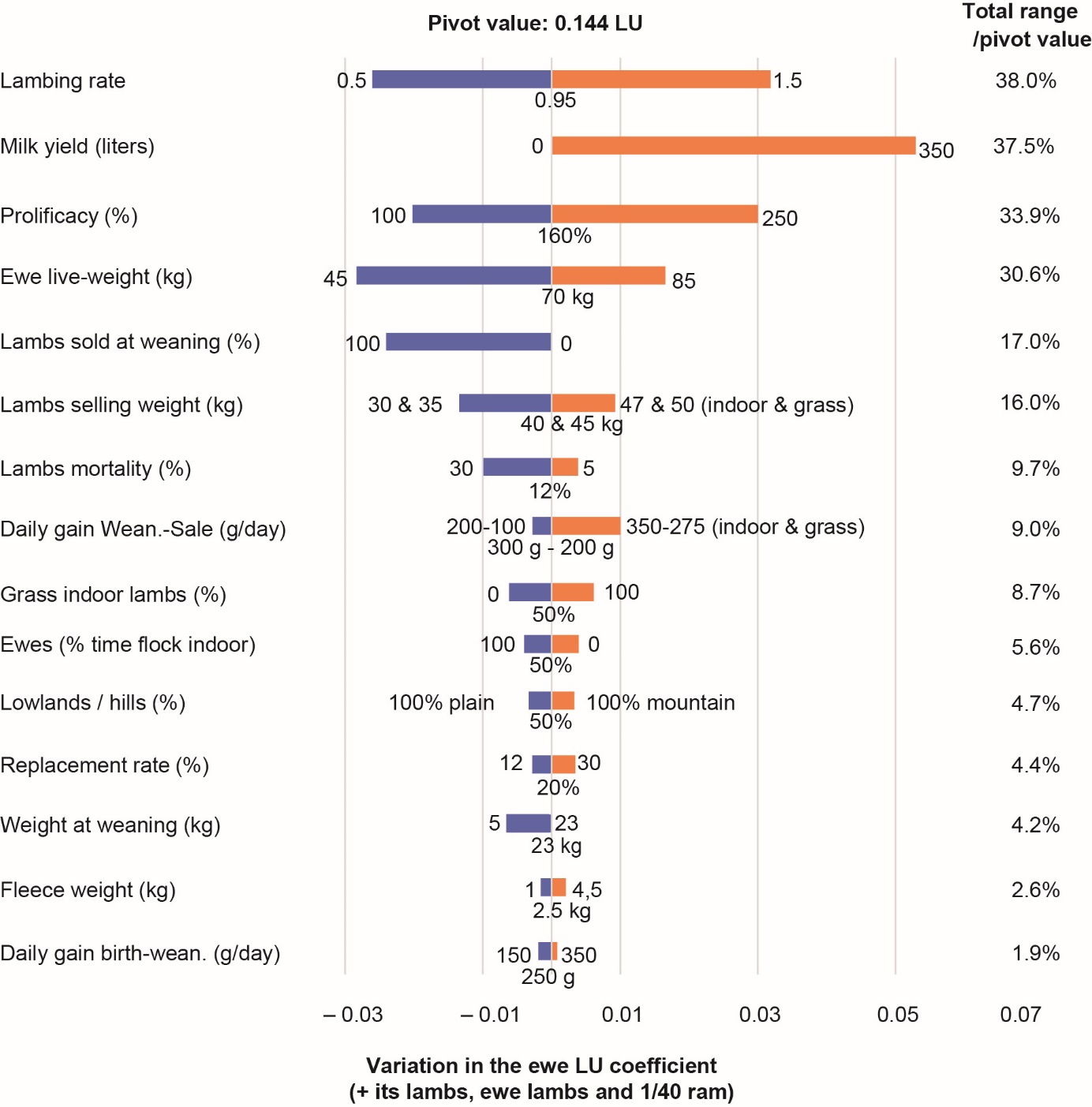
Variables ranked in descending order of impact on the pivotal LU value defined for an average animal whose characteristics are specified as the central value of each variable (e.g., lambing rate of 0.95).
We thus propose Equation (13) for the “followed ewe” (ewes plus lambs plus rams), considering the presence of one ram for every 40 ewes and the live weight of the ram 40% higher than that of the ewe:
(13) NEt_ewe (MJ/year) =90.3×LW0.75+5.1×LW+4.37×QM+EP×(365.1×(1-%SW)+427.6)+317
where LW is the weight of the ewe, QM is the quantity of milk milked, EP is the ewe productivity and %SW is the proportion of lambs sold at weaning.
To obtain the LU value of the flock, the NEt_ewe value (Equation (13)) must be divided by 29 000 and multiplied by the yearly average number of ewes in the flock.
Although we have proposed a global equation including lambs fattened on-farm, we propose the elements below for situations where lambs would be purchased to be fattened on-farm. The calculation of their LU value accounts for the maintenance, activity and growth requirements (Equations 10.3, 10.5 and 10.7, respectively, IPCC, 2019). Equation (14) proposes the calculation of the NEt requirement of a lamb over its wean-to-sale period.
(14) NEt_ Lamb (MJ/head)=(SW-WW)×(0.5×(0.393×DG+0.0138)×(SW+WW)+0.1403×(SW+WW)0.75+ 2.775×DG)/DG
where SW is sale weight, WW is weaning (or purchase) weight, and DG is average daily weight gain (kg/d).
We propose some figures for standard types of lambs. They are contrasted in terms of weight and fattening methods (Table 9). As the duration of presence of these lambs is generally less than one year, we also calculate the LU coefficient on the basis of a 365-day presence.
Table 9. Characteristics and LU coefficients of four types of fattened lambs.
Characteristics of the lambs |
Indoor fattening |
On-grass fattening |
||
|---|---|---|---|---|
Live weight for sale (kg) |
33 |
40 |
40 |
48 |
Average daily gain (g.d-1) |
350 |
350 |
225 |
225 |
Live weight at weaning (kg) |
23 |
23 |
23 |
23 |
Age at sale (days) |
104 |
124 |
151 |
186 |
Net Energy Requirement (MJ) |
222 |
416 |
514 |
831 |
Livestock unit value over |
0.008 |
0.014 |
0.018 |
0.029 |
Annual livestock unit coefficient |
0.098 |
0.108 |
0.086 |
0.094 |
2.3 Goats
Following the same approach as for sheep, we prioritize the variables taken into account in the calculation of goat net energy requirements (Figure 3). As kids are usually fattened in a separate enterprise, we isolate the calculation of the kid's LU after weaning from that of its dam, accounting for the weaning-sale period. The LU value of the replacement goat kids is integrated into the LU value of the goats. Three variables cause the pivotal value to vary by more than 10% when they vary between the minimum and maximum values used (Figure 3).
Figure 3. Variations in the LU coefficient of the goat, generated by the variation of the variables entering the calculation of the net energy requirements between the minimum and maximum values retained.
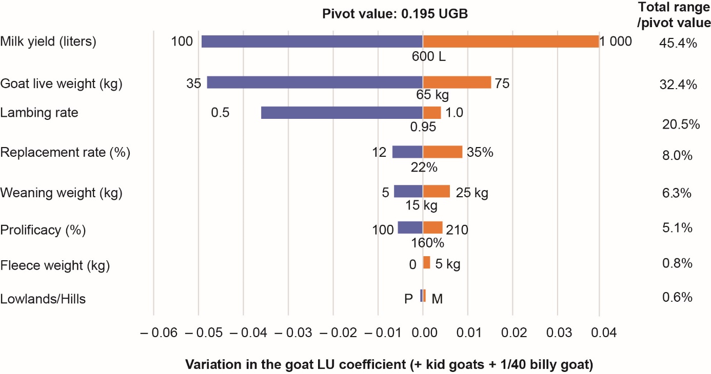
Variables ranked in descending order of impact on the pivotal LU value defined for an average animal whose characteristics are specified as the central value of each variable (e.g., milk production of 600 litres)
We integrate these three variables into the equation for calculating the NEt (MJ/year) for goats:
(15) NEt_Goat (MJ/year)=(115.0+12.23×LR)×LW0.75+(3.0×QM+234)×LR+4.6×LW+431
where LR is the kidding rate (number of kids per goat per year), LW is the average live weight and QM is the amount of milk produced per goat per year (including milk drunk by kids).
Note that this equation is also well adapted for long lactation herds (beyond one year or even two years) by always considering the annual milk production of the herd per goat (the LU concept being based on a one-year campaign); the kidding rate can then be reduced to 0.3 or 0.4 at the herd level. As LR is the variable that induces the least variability in the calculation and its range of variation is a priori low, we set it at 0.95 to propose the simplified Equation (16):
(16) NEt_Goat (MJ/year)=126.6×LW0.75+4.6×LW+2.85×QM+653
For a billy goat, the proposed equation is of the same type as that used for rams, i.e.
(17) NEt_BillyG (MJ/year)=115.0×LW0.75+4.6×LW
where LW is the weight of the billy goat.
As for sheep, we propose a simplified global Equation (18) for a “followed goat” (goats, replacement, and billy goat) considering that the weight of billy goats is 40% higher than that of goats and that there is one billy goat present for 40 goats. The energy requirement of any fattened kids is additional.
(18) NEt_Goat (MJ/year)=130.3×LW0.75+4.75×LW+2.85×QM+653
where LW is the average weight of the goat and QM is the amount of milk produced per goat per year.
To obtain the herd's LU value, the NEt_Goat value (Equation (18)) must be divided by 29,000 and multiplied by the average number of goats over one year old in the herd.
As for other animals, the LU value of kids takes into account activity, maintenance and growth requirements (Equations 10.3, 10.5 and 10.7, respectively, IPCC, 2019). The calculation parameters concern the weaning and end of fattening period weights of the animal and its average growth rate. We take the situation of an indoor fattening. The equation for the total net energy requirement of the kid during its post-weaning rearing period is as follows:
(19) NEt_kid (MJ/head)=(LW-WW)×[0.5×(0.33×DG+0.0067)×(LW+WW)+0.1873×(LW+ WW)0.75+5×DG]/DG
where WW is the starting live weight (usually weaning weight), LW is the sale weight and DG is the average daily weight gain (kg/d).
For a quicker calculation for typical situations, we present (Table 10) the net energy requirements of the animals for the weaning-to-sale period (or one year), as well as the LU values, by varying the age and weights at weaning and sale.
Table 10. Characteristics and LU coefficients of seven types of fattened kids differing in age at weaning and duration of fattening period.
Duration of the period (days) |
25 |
49 |
76 |
55 |
36 |
55 |
319 |
|---|---|---|---|---|---|---|---|
Age at end of period (days) |
27 |
51 |
78 |
80 |
82 |
101 |
365 |
Live weight end of period (kg) |
11 |
17.5 |
25 |
25 |
25 |
25 |
50 |
Average daily gain (g.d-1) |
275 |
180 |
110 |
||||
Age at weaning (days) |
2 |
2 |
2 |
25 |
46 |
46 |
46 |
Live weight at weaning (kg) |
4 |
4 |
4 |
10 |
15 |
15 |
15 |
Net Energy Requirement (MJ) |
90 |
211 |
392 |
315 |
229 |
289 |
1989 |
Livestock unit value over the period |
0.003 |
0.007 |
0.014 |
0.011 |
0.008 |
0.010 |
0.069 |
Annual livestock unit coefficient |
0.044 |
0.054 |
0.065 |
0.073 |
0.079 |
0.065 |
0.078 |
3. Discussion
3.1. The concept of the Livestock Unit
The evolution over the years of the definitions and uses of the LU concept makes its use hazardous for studies of the performance of livestock systems, particularly in view of the challenges of optimizing the resources used by the animals and for the purposes of comparing the "weight" of livestock in production systems. By returning to the initial concept of the LU, which linked it to the energy requirements of the animals, we propose an objective and measurable unit for all types of ruminant animals. The proposed equations take into account the main variables determining the net energy requirement of animals, including weight and production level. These parameters vary from one farm to another but are readily available and can lead to LU values varying by a factor of two for two animals of the same category; for example, until now, all dairy cows counted as 1 LU, whereas with our proposal, a 500 kg dairy cow producing 3 000 L of milk per year would count as 0.90 LU compared to 1.87 LU for a 780 kg cow producing 10 000 L of milk. We retain the notion of one reference animal for one LU, with an overall net annual energy requirement of 29 000 MJ. This proposal, established initially for ruminant farms, could be extended to farms with other types of herbivores and to monogastric animals.
This new definition of the livestock unit makes it possible to address questions relating to the use of total feed resources (fodder, concentrates, coproducts) used to meet the energy requirements of the animals, which is consistent with the evolution of the ruminant diet, which often includes a significant proportion of concentrates. However, the annual dry matter intake of animals could be estimated. The IPCC proposes three equations (10.14, 10.15 and 10.16) to estimate the gross energy requirements of animals from the net energy requirements and the estimated digestibility of the gross energy of the ration. Dry matter intake can then be obtained by dividing the gross energy requirement by the gross energy content of the ration. This method allows very large-scale estimates to be made for national inventories of animal intake of fodder. However, the estimates of ration digestibility are too coarse, and they do not take into account the interactions between the feeds making up the ration, so they cannot be used at the farm level.
The use of the IPCC reference system makes it possible to i) take into account the specificity of animal management, which has repercussions on energy requirements and therefore on the resources mobilized (even if we cannot go as far as to evaluate them); ii) make the equations general and applicable on a global scale; iii) make them relatively easy to implement by isolating the variables that determine the result, which are available on the farm.
3.2 Choice of key variables in the proposed equations
The variables of live weight and animal productivity (milk, prolificacy, growth rate) are among the most important determinants of the animals' net energy requirements (INRA, 2018) and therefore of their LU coefficients. We confirmed their importance after the analysis of the impact of the potential variation of each variable, taken individually, on the variation in LU coefficients. It would have been theoretically necessary to cross-check the variability of some variables because they are not all independent of each other. For example, the weight of Holstein dairy cows may be positively correlated with milk production (Berry et al., 2007), while increasing the weight of suckler cows may have a negative impact on cow productivity and calf weight (Farrell et al., 2021). For sheep, we considered some correlations, such as the impact of lamb birth mode (single, double) and dam weight on lamb birth weight, and thus expected weight gain before sale. However, other links exist: for sheep, the mortality rate of lambs is partly linked to the level of prolificacy, and the growth rate of lambs is also partly linked to the method of fattening in buildings, i.e., with concentrates, or on grass, on more or less productive surfaces; the weight at weaning and the share of lambs sold at weaning are highly correlated with, in specialized dairy sheep farming, lambs weaned very young to be fattened off the farm.
The variables that we have retained in our proposed equations, in particular the weight of the animal and its level of production, appear on the one hand to be determining factors in the LU value and, on the other hand, their values can be approximated without too much difficulty. A more precise sensitivity study, taking into account all the links between variables, would be difficult to implement and would come up against the availability of data and the multiplicity of situations encountered (e.g., linking the level of growth of the animals with the proportion and characteristics of the grass grazed, which changes over time).
Furthermore, the sensitivity analysis was carried out on the basis of ranges of variation of zootechnical parameters rather specific to OECD countries, i.e., not covering certain more extreme situations in terms of, for example, the size or production level of animals with different genotypes. The proposed equations would not necessarily be challenged, but their range of validity must be restricted to the tested ranges of variation, and some additional components of net energy requirements could be taken into account (e.g., the work done by draught animals).
3.3. The new LU values calculated
The proposed LU values for the different animal categories studied are sometimes quite far from historical values, especially for dairy cattle since their level of milk production, which has a strong impact, has a potentially large range of variation. The deviations from historical values are smaller for suckler cattle but higher for suckler sheep.
We propose to compare the results of different methods for calculating LU coefficients for dairy cattle on the one hand and sheep for meat on the other. The values from four methods are compared: i) historical method (MH); ii) method based on the full IPCC equations (IPCC, 2019) (MIPCC); iii) "complete" method MC and iv) "simplified" method MS, both based on the equations proposed in Part 2 of this article. To judge the adaptation of the two proposed methods to a wide range of contexts, we use very contrasting farming systems (production level and animal size) for each of the two types of production studied (Tables 11 and 12). These systems are taken from the French farm-types proposed by the Institut de l'Elevage (IDELE-bovins-lait, 2021, IDELE-Ovins, 2021).
Table 11. Main characteristics of three contrasting French dairy cattle systems in terms of breed and weight of cows, production level, access to pasture, age at first calving and type of males sold.
Case name |
Breed |
Weight |
Milk/cow |
Fat (%) |
Grazing period |
Age at |
Males sold |
|---|---|---|---|---|---|---|---|
Specialized milk |
Holstein |
680 |
9 950 |
40.0 |
0 |
28 |
Calves |
Milk + steers |
Normande |
720 |
6 000 |
42.0 |
4.5 |
29 |
Steers |
Alpine milk zone |
Tarine |
545 |
4 185 |
35.6 |
5.5 including |
36 |
Calves |
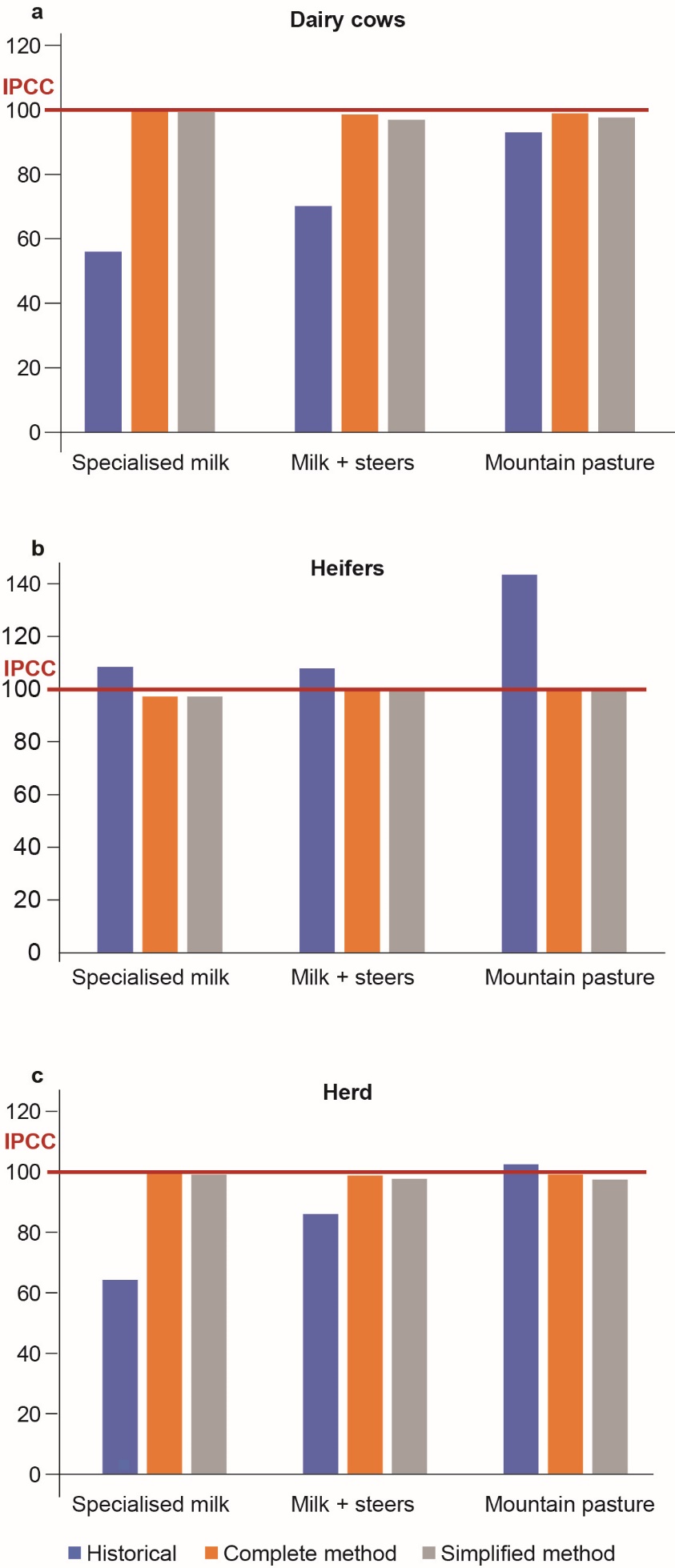
The LU coefficient of the dairy cows calculated according to Mc (Equation (1)) or Ms (Equation (2)) is very close to that of MIPCC, with a maximum difference of 3% between MIPPC and Ms for the Normand farm-type, linked to the milk fat content of the Normand breed and to the duration of grazing not taken into account in Ms. The significant difference with the historical value of 1 LU is explained by taking into account the level of milk production. Logically, the difference is greatest in the case of the specialized herd producing 9 950 litres/cow/year (+44%) and smallest for the alpine milk system at 4,185 litres/cow/year (+7%). The proposed method for calculating LU coefficients for breeding heifers provides results very close to MIPCC (no more than 3% difference), but the values are lower than historical coefficients (Figure 4b). For systems with a relatively heavy breed (Holstein or Normande) and with an age at first calving of less than 30 months, the difference in the LU value of the breeding heifers is –8% on average between MIPCC and the historical coefficients. On the other hand, for a smaller cow size (and therefore smaller heifers) and a calving age of primiparous cows at 36 months (and therefore a lower daily growth from birth to calving), the difference is –43% for the Tarine breed alpine system. It should be noted that for 33-month-old Normand steers, the LU coefficients obtained by MIPCC and MC are very close (less than 3% difference) but 19% lower than historical values (same reasons as for heifers). In the end, the numbers of total LUs of the herds calculated according to the Mc or Ms methods are very close to those obtained by MIPCC (Figure 4c) with less than a 3% difference for the three dairy systems studied. The difference with the historical coefficients remains significant for the most productive system per cow (+36%) and diminishes when the level of cow production approaches the historical reference of 3,000 litres/cow/year.
Figure 4: Deviation of the LU values of dairy cows (a), breeding heifers (b) and the whole herd (c) for the three types of dairy farms described in Table 11, calculated according to the historical, complete and simplified methods, in relation to a base 100 corresponding to the calculation of LUs according to the IPCC equations.
For the meat sheep systems studied, the characteristics of which are presented in Table 12, Figure 5a shows that MH gives a result that is on average 26% higher than MIPCC for a “followed ewe”, with in particular a very high difference (51%) for Case 3 where the ewes have low weight and productivity. This overevaluation concerns the ewes (Figure 5b), since the LU value of the lambs is on the contrary underevaluated on average by 21% by MH (Figure 5c). MC is very close to MIPCC, with an average of 1% undervaluation for the “followed ewe”, linked to Case 3, whose ewes are in full grazing, with important energy needs in this context (variable not taken into account in MC). MC takes well into account the needs of the lambs. MS gives on average a result 7% higher than MIPCC for the “followed ewe”, with less precise results than MC for the lambs (amplitude from –12 to +26% compared to MIPCC according to the four systems, vs. - 3 to +6% only for MC), the needs of the ewes being well approached.
Table 12. Main characteristics of four contrasting French meat sheep systems in terms of ewe weight, ewe productivity and rearing method and characteristics of lambs sold.
Name of case |
Ewe weight (kg) |
Replac. rate (%) |
Lambing rate |
Prolif. (%) |
Lambs mortal. (%) |
Ewe prod. |
lambsweight (kg) |
Daily Gain W-Sales |
Sale at weaning |
Indoor lambs (%) |
|
|---|---|---|---|---|---|---|---|---|---|---|---|
Case 1 |
Prolific, plain |
70 |
18 |
1.07 |
208 |
16 |
1.87 |
33.7 |
275 g |
0 |
100 |
Case 2 |
West. Semi-ext. |
85 |
20 |
0.96 |
172 |
15 |
1.40 |
37.0 |
210 g |
0 |
46 |
Case 3 |
Pastor., Pre-Alps |
50 |
19 |
0.78 |
117 |
12 |
0.80 |
35.0 |
70 g |
46% |
0 |
Case 4 |
Mountain, grass |
70 |
20 |
0.95 |
156 |
9 |
1.35 |
32.5 |
270 g |
0 |
100 |
Figure 5. Deviation for 4 types of sheep farming described in Table 12 of the LU values of the “followed” ewe (+ lambs and ram) (a), single ewe (b), lambs (c), calculated according to the historical, complete and simplified methods, compared to a base 100 corresponding to the calculation of LU according to the IPCC equations.
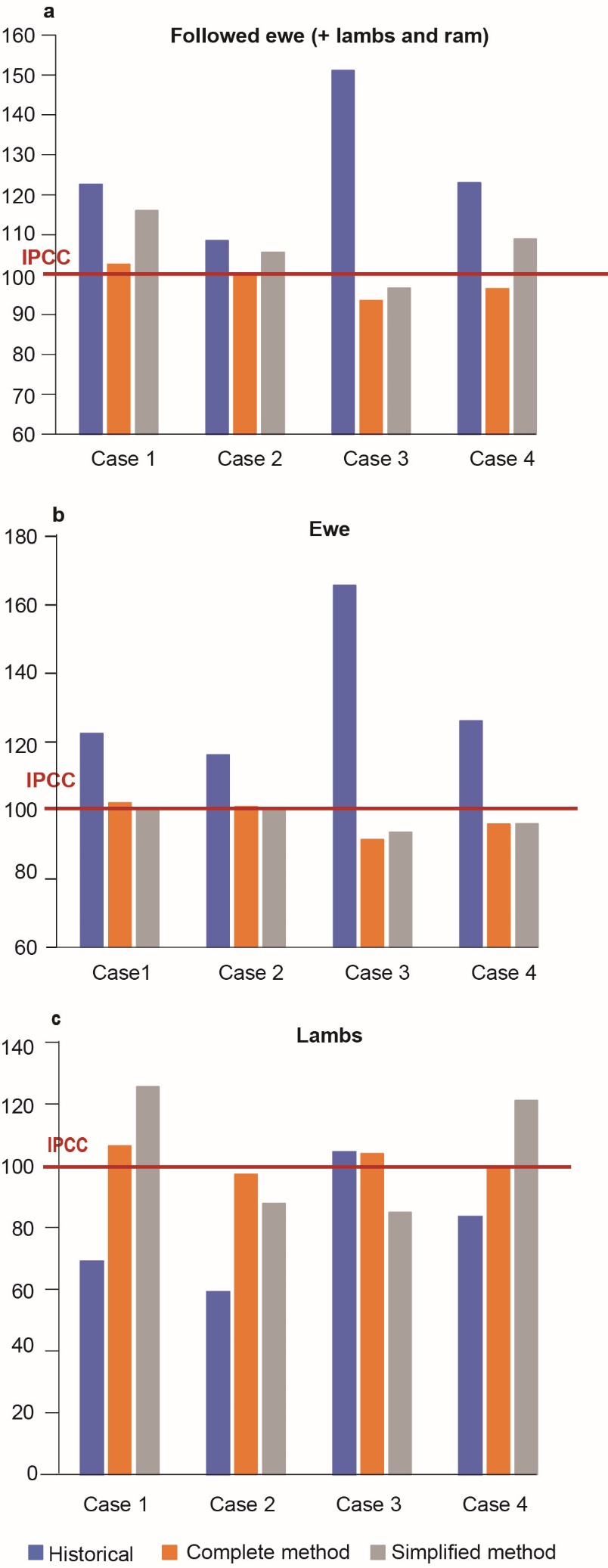
Note that the LU value of the lambs for the historical method is evaluated on the basis of an LU coefficient of 0.05 for an attendance time of 130 days (including the preweaning period).
Furthermore, for dairy ewes, the average values derived from Mc and Ms remain of the same order as with MH. For example, for a 70 kg ewe producing 280 kg of milk per year, with her lambs weaned at 10 kg, the LU coefficient (Mc) is 0.17, comparable to that calculated by the Institut de l'Élevage (France) for ewes of the same type (Idele, 2014a). Similarly, in goat production, the orders of magnitude correspond to the usual standards for relatively productive production systems (963 litres of milk per goat in France in 2019, Idele, 2020b).
For suckler cattle, considering the weight of the animals is a fundamental element in refining the calculation of the LU value of the herds and the indicators used, which may lead to questioning certain conclusions established on the basis of historical LU coefficients. For example, Veysset et al. (2014) published a study on the long-term evolution of the performance of beef farms. Using the sample data used, over the period 1991-2016 (26 years), we calculated the average weight of all cull cows marketed (n=29 626, for 2 143 farm-years, with a maximum number of 95 farms in 1991). This increased by 15.2% between 1991-1992 and 2015-2016 (678 and 781 kg live/head, respectively). This weight gain translates into an 8.4% increase in the LU value of cows, which represent 50 to 60% of the herd's LUs depending on the system. As a result, the stocking rate (number of total livestock units in the herd per ha of forage area), which, with the historical method of calculating livestock units, was announced as decreasing by 6.5% over the period studied, would increase with the proposed new calculation method. Furthermore, while the analysis concluded that meat production per LU, the result of technical and genetic progress, would increase by 8.0%, it could be stable or even decrease if the new method of calculating LUs, which takes into account the increase in cow weight, is used.
Conclusion
Quantifying the size of herds, which is used in various types of work, requires the definition of an animal unit to make comparisons between farms, regions or countries, and over time. The historical approach to the concept of LU proposes very simple and standardized equivalences by species and by major types of animals; this approach is still suitable for large-scale statistical purposes, but it appears too crude for technical and economic studies at the sub-level, particularly at the farm level.
The use of the concept of net energy requirements of animals is transverse to livestock species and for different types of production. It thus makes it possible to study livestock systems that vary in terms of technical functioning, animal production levels and the genotypes used. We therefore propose to use this concept of net energy requirements as the basis for calculating LUs, using the equations published by the IPCC. For very fine approaches, it is possible to systematically use these equations if all the necessary parameters are available. This method makes it possible to consider all energy requirements, including those related to animal work, and even other regional specificities, such as the type of grazing. In this paper, we propose two intermediate methods between the full application of these IPCC equations and the very standardized historical method. These two methods take into account, among other things, the two variables that explain the most important part of the potential differences in animal needs, namely, their weight and their production level. The first of the two methods attempts to approximate the IPCC equations as closely as possible but, following a sensitivity analysis, leaves out certain parameters that have little impact and are not easy to monitor properly on most farms. We propose a second "simplified" method, taking into account only the most important and easily accessible parameters. Compared to the historical approach, these two methods allow a better discrimination of the influence of the format and the level of production on the animal stocking rate while remaining applicable to large scales (pool of several hundred farms, territories, etc.).
For many applications and research work in particular, the use of one or the other of these two methods should make it possible to better translate the differences in animal stocking rate in relation to the feed requirements of the animals, particularly in comparative studies between farms or diachronically. Even if our proposal does not directly address the question of the resources needed to raise a type of animal and for its production, from a qualitative and quantitative point of view, it does address the question of the level of needs to be met by bringing them closer to the farm's production capacity of plant resources for its herds.
This article aims to provide elements for thought and a concrete proposal for new equations adapted to studies on the evaluation of ruminant farming systems. Given the important issues raised, this contribution should be discussed within a consortium of researchers and users to strengthen or even complete these proposals. It would also be necessary to pursue this approach for monogastric species, which are unfortunately not currently taken into account by the IPCC.
Acknowledgements
This methodological proposal is the result of the European project MIX-ENABLE, which benefited from the financial support of the participating states (including France) and the European Commission, through the H2020 ERA-NET CORE Organic Cofund programme. We would like to thank Jacques Agabriel for his attentive and wise reading, as well as the reviewers of the INRAE Productions Animales journal.
References
- Assouma M.H., Lecomte P., Hiernaux P., Ickowicz A., Corniaux C., Decruyenaere V., Diarra A.R., Vayssières J., 2018. How to better account for livestock diversity and fodder seasonality in assessing the fodder intake of livestock grazing semi-arid sub-Saharan Africa rangelands. Livest. Sci., 216, 16-23. doi:10.1016/j.livsci.2018.07.002
- Benoit M., Sabatier R., Lasseur J., Creighton P., Dumont B., 2019. Optimising economic and environmental performances of sheep-meat farms does not fully fit with the meat industry demands. Agron. Sustain. Dev., 39, pp.40. doi:10.1007/s13593-019-0588-9
- Berry D.P., Buckley F., Dillon P., 2007. Body condition score and live-weight effects on milk production in Irish Holstein-Friesian dairy cows. Animal, 1, 1351-1359. doi:10.1017/S1751731107000419
- Blaxter K.L., 1989. Energy metabolism in animals and man. Cambridge University Press, 305p.
- Boichard J., 1969. Gestion agricole et géographie rurale. Revue de géographie de Lyon 44, 323-374. doi:10.3406/geoca.1969.2647
- Cavailhès J., Bonnemaire J., Raichon C., Delamarche F., 1987. Caracteres regionaux de l'histoire de l'elevage en France. 1-Méthodographie et résultats statistiques 1938-1980., 636p.
- Coléou J., 1960. Les références concernant le rationnement des animaux. Le bilan fourrager. Écon. Rurale, 43, 33-54. doi:10.3406/ecoru.1960.1690
- Demarquilly C., Faverdin P., Geay Y., Vérité R., Vermorel M., 1996. Bases rationnelles de l'alimentation des ruminants. INRA Prod. Anim., 71.80. doi:10.20870/productions-animales.1996.9.HS.4089
- Drennan M.J., McGee M., 2009. Performance of spring-calving beef suckler cows and their progeny to slaughter on intensive and extensive grassland management systems. Livest. Sci., 120, 1-12. doi:10.1016/j.livsci.2008.04.013
- EUROSTAT, 2019. Unités Gros Bétail (UGB). Coefficients. Statistics Explained. https://ec.europa.eu/eurostat/statistics-explained/index.php?title=Glossary:Livestock_unit_(LSU)
- Farrell L.J., Morris S.T., Kenyon P.R., Tozer P.R., 2021. Simulating Beef Cattle Herd Productivity with Varying Cow Liveweight and Fixed Feed Supply. Agriculture 11, 35. doi:10.3390/agriculture11010035
- IDEA, 2019. Table de conversion des UGB alimentaires annuelles pour le calcul de l'indicateur A 10. https://idea.chlorofil.fr/utilisation/outils-dapplication.html
- IDELE-bovins-lait, 2021. http://idele.fr/no_cache/recherche/publication/idelesolr/recommends/cas-types-bovins-lait.html Consulté le 6 juillet 2021.
- IDELE-Ovins, 2021. http://idele.fr/no_cache/recherche/publication/idelesolr/recommends/cas-types-ovins-allaitants.html.Consulté le 6 juillet 2021.
- Idele, 2010. Engraisser des bovins en Rhône-Alpes, itinéraires techniques types. Institut de l'Élevage, Réseaux d'élevage, Chambres d'Agriculture Rhône-Alpes PACA, Paris, 29p.
- Idele, 2014a. Alimentation des ovins : rations moyennes et niveaux d'autonomie alimentaires. Collection résultats, 54p.
- Idele, 2014b. Guide de l'alimentation du troupeau bovin allaitant. Vaches, veaux et génisses de renouvellement. Collection les Incontournables. Institut de l'Élevage, Paris, France, 340p.
- Idele, 2019. Systèmes bovins laitiers des zones de montagnes et piémonts d'Auvergne et de Lozère - conjoncture 2019. 142p.
- Idele, 2020a. Les chiffres clés du GEB, bovins 2019, productions lait et viande. Institut de l'Élevage et CNE, Paris, France, 12p.
- Idele, 2020b. Résultats de controle laitier - Espèce caprine - France 2019. France conseil élevage, collection résultats, 34p.
- Idele, 2020c. Résultats de contrôle laitier, espèce bovine, France 2019. Collection Résultats, Institut de l'Élevage, Paris, France, 115p.
- Idele, 2020d. Résultats du contrôle des performances bovins allaitants, France 2019. Collection Résultats, Institut de l'Élevage, Paris, France, 128p.
- Iger-Centres-de-Gestion, 1989. Le mot juste. 250 termes et expressions pour analyser les résultats de gestion des exploitations d'élevage. 168p.
- INRA, 2018. Alimentation des ruminants. Éditions Quae, Paris, France, 728p
- IPCC, 2019. 2019 Refinement to the 2006 IPCC Guidelines for National Greenhouse Gas Inventories. Chapter 10. Emissions From Livestock And Manure Management. 209p
- Jahnke H.E.,1982. Livestock production systems and livestock development in Tropical Africa. Kieler Wisserschaftverlag Vauk, Germany, 273p.
- Lampert V.N., Canozzi M.E.A., McManus C.M., Dill M.D., de Oliveira T.E., Mercio T.Z., Teixeira O.S., Barcellos J.O.J., 2020. Modelling beef cattle production systems from the Pampas in Brazil to assess intensification options. Sci. Agric., 77, 13p. doi:10.1590/1678-992x-2018-0263
- McLaren C., 1997. Dry Sheep Equivalents for comparing different classes of livestock. Information notes. Department of Primary industries., https://www.researchgate.net/publication/242130820_Dry_Sheep_Equivalents_for_Comparing_Different_Classes_of_Livestock.
- Murphy B., Crosson P., Kelly A.K., Prendiville R., 2018. Performance, profitability and greenhouse gas emissions of alternative finishing strategies for Holstein-Friesian bulls and steers. Animal, 12, 2391-2400. doi:10.1017/S1751731118000034
- Office de l'élevage, 2008. Production de jeunes bovins de races à viande et de races laitière, 13 fiches de références sur les itinéraires techniques. Institut de l'Élevage, Chambres d'Agriculture Pays de la Loire et Bretagne, Arvelis Institut du Végétal, Paris, France, 37p.
- Ortigues I., 1991. Adaptation du métabolisme énergétique des ruminants à la sous-alimentation. Quantification au niveau de l'animal entier et de tissus corporel. Reprod. Nutr. Dev., EDP Sciences, 31, 593-616.
- Pesonen M., Honkavaaea M., Huuskonen A., 2013. Production, carcass and meat quality traits of Hereford, Charolais and HerefordxCharolais bulls offered grass silage-grain-based rations and slaughtered at high carcass weights. Acta Agricult. Scand., Section A 63, 28-38. doi:10.1080/09064702.2013.777091
- Pravia M.I., Ravagnolo O., Urioste J.I., Garrick D.J., 2014. Identification of breeding objectives using a bioeconomic model for a beef cattle production system in Uruguay. Livest. Sci.,160, 21-28. doi:10.1016/j.livsci.2013.12.006
- Réseaux d'élevage, 2005. Produire des bœufs dans l'Est, 7 itinéraires techniques. Institut de l'Élevage, Chambres Régionales d'Agriculture d'Alsace, de Lorraine et de Champagne-Ardenne, 18p.
- Rothman-Ostrow P., Gilbert W., Rushton J., 2020. Tropical Livestock Units: Re-evaluating a Methodology. Front Vet. Sci., 7, 556788.
- Scarnecchia D.,1985. The Animal-Unit and Animal-Unit-Equivalent Concepts in Range Science. J. Range Manage., 38, 346-349. doi:10.2307/3899419
- Scarnecchia D., Kothmann M., 1982. A dynamic approach to grazing management terminology. J. Range Manage., 35, 262-264. doi:10.2307/3898407
- Sepchat B., Dhour P., Agabriel J., 2017. Production laitière des vaches allaitantes : caractérisation et étude des principaux facteurs de variation. In : Élevage bovin allaitant. Agabriel J., Renand G., Baumont R. (Eds). Dossier, INRA Prod. Anim., 30, 139-152. doi:10.20870/productions-animales.2017.30.2.2240
- Taylor R.F., Crosson P., Kelly A.K., McGee M., 2018. Benchmarking technical and economic performance of beef cow-calf to finishing production systems in Ireland. Prof. Anim. Scient., 34, 421-434.
- Thériez M., 1991. Conséquences de l'augmentation de la prolificité sur l'élevage des agneaux et sur la production de viande. INRA Prod. Anim., 4, 161-168. doi:10.20870/productions-animales.1991.4.2.4328
- Upton M., 1989. Livestock productivity assessment and herd growth models. Agric. Syst., 29, 149-164. doi:10.1016/0308-521X(89)90060-7
- Upton M., 1993. Livetock productivity assessment and modelling. Agric. Syst. 43, 459-472. doi:10.1016/0308-521X(93)90034-Y
- Veysset P., Benoit M., Laignel G., Bebin D., Roulenc M., Lherm M., 2014. Analyse et déterminants de l'évolution des performances d'élevages bovins et ovins allaitants en zones défavorisées de 1990 à 2012. In : Spécificités de l'élevage de ruminants en montagne. Grosclaude J., Thibier M., Baumont R. (Eds). Dossier, Inra Prod. Anim., 27. 49-63. doi:10.20870/productions-animales.2014.27.1.3054
Abstract
Originally based on the ingestion of forage by herbivores and by extension on their energy requirements, the concept of Livestock Unit (LU) is widely used, without always being precisely defined, to study livestock systems. However, the calculation of the LU value of a given animal can be considered as quite rough since it does not take into account its size, production level, nor its rearing conditions, on which its energy and thus feed requirements depend. We propose a LU calculation adapted to the bovine, ovine and caprine species based on the net energy needs of the animals, using the IPCC (Intergovernmental Panel on Climate Change) equations and parameters. Thanks to a sensitivity analysis of these parameters, we confirm that the weight of the animals and their production level are determinants of their net energy requirements. By integrating these two parameters, we propose two types of equations that differ in their level of precision and in the availability of the required data. Based on an equivalence of 29 000 MJ for a LU represented by a 600 kg dairy cow producing 3 000 kg of milk per year with a 4 % fat, we keep the notion of reference animal. The proposal allows taking into account, through the size of the animals, their production level and their genotype, the variability of the animals' feed requirements. The LU coefficients calculated in this way can differ significantly from historical coefficients and thus modify the conclusions of comparisons of farming systems between themselves or over time.
Attachments
No supporting information for this articleArticle statistics
 Views: 64890
Downloads
 PDF: 9018
 XML: 112
Most read articles by the same author(s)
- Sarah LAISSE, René BAUMONT, Léonie DUSART, Didier GAUDRÉ, Benoit ROUILLÉ, Marc BENOIT, Patrick VEYSSET, Didier RÉMOND, Jean-Louis PEYRAUD, The net feed conversion efficiency of livestock: a new approach to assess the contribution of livestock to human feeding , INRAE Productions Animales: Vol. 31 No. 3 (2018): Volume 31: Issue3: Dossier: Feed resources for livestock
- Bertrand DUMONT, Sylvie COURNUT, Claire MOSNIER, Sylvie MUGNIER, Géraldine FLEURANCE, Geneviève BIGOT, Louise FORTEAU, Patrick VEYSSET, Hélène RAPEY, Understanding the benefits of herbivore system diversification: lessons from French Massif central , INRAE Productions Animales: Vol. 33 No. 3 (2020)
- Christian DUCROT, Maria Belén BARRIO, Alain BOISSY, François CHARRIER, Sergine EVEN, Pierre MORMÈDE, Sandrine PETIT, Marie-Hélène PINARD-VAN DER LAAN, François SCHELCHER, François CASABIANCA, Alain DUCOS, Gilles FOUCRAS, Raphaël GUATTEO, Jean-Louis PEYRAUD, Muriel VAYSSIER-TAUSSAT, Patrick VEYSSET, Nicolas C. FRIGGENS, Xavier FERNANDEZ, Jointly improving animal health and welfare in the transition of livestock systems towards sustainability , INRAE Productions Animales: Vol. 37 No. 3 (2024)
- Bertrand DUMONT, Marc BENOIT, Sophie CHAUVAT, Sylvie COURNUT, Guillaume MARTIN, Pierre MISCHLER, Marie-Angelina MAGNE, Sustainability of multi-species livestock farms in France and Europe: benefits, obstacles and levers for their scaling-out , INRAE Productions Animales: Vol. 36 No. 1 (2023)
- Marc BENOIT, Pietro BARBIERI, Bertrand DUMONT, What type of livestock farming for a successful organic agriculture in the Anthropocene era? , INRAE Productions Animales: Vol. 37 No. 2 (2024): Special issue: Organic livestock farming: conditions and potential for development
- Marc BENOIT, Lucille STEINMETZ, Dorian FLÉCHET, Laurent PIET, Thomas POMEON, Organic livestock farming in France: farm structure, spatial distribution and recent trends , INRAE Productions Animales: Vol. 37 No. 2 (2024): Special issue: Organic livestock farming: conditions and potential for development
- Vincent CHATELLIER, Christophe PERROT, Emmanuel BEGUIN, Marc MORAINE, Patrick VEYSSET, Competitiveness and production jobs in the French bovine sectors , INRAE Productions Animales: Vol. 33 No. 4 (2020)
- Marie-Odile NOZIÈRES-PETIT, Yuna CHIFFOLEAU, Patrick VEYSSET, Producing and marketing of organic animal products: a driving force for the agroecological transition? , INRAE Productions Animales: Vol. 37 No. 2 (2024): Special issue: Organic livestock farming: conditions and potential for development
- Larissa MYSKO, Jean-Joseph MINVIEL, Patrick VEYSSET, Isabelle VEISSIER, Relationships between economic performance, environmental performance and animal welfare , INRAE Productions Animales: Vol. 38 No. 4 (2025): Animal welfare: scientific advances and innovations for sustainable livestock farming systems